最小二乘法多项式曲线拟合及其python实现
- 多项式曲线拟合问题描述
- 最小二乘法
- 针对overfitting,加入正则项
- python实现
- 运行结果
多项式曲线拟合问题描述
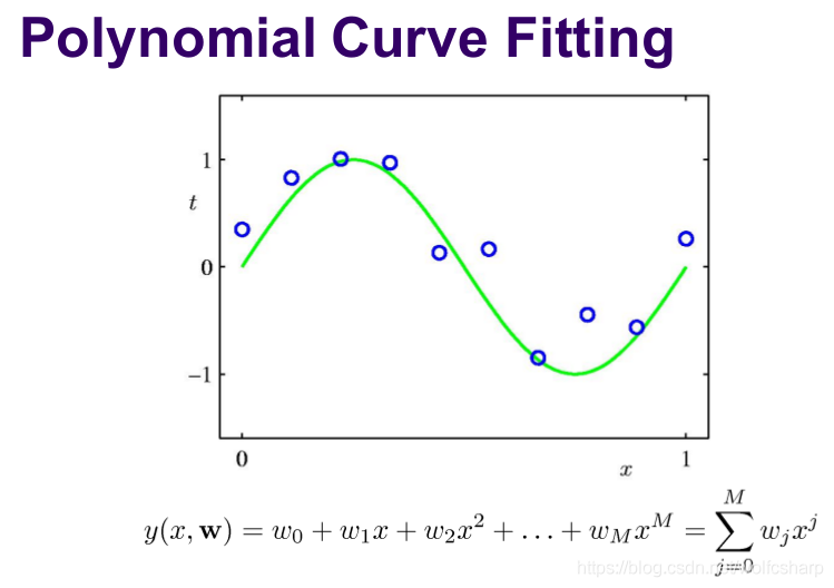
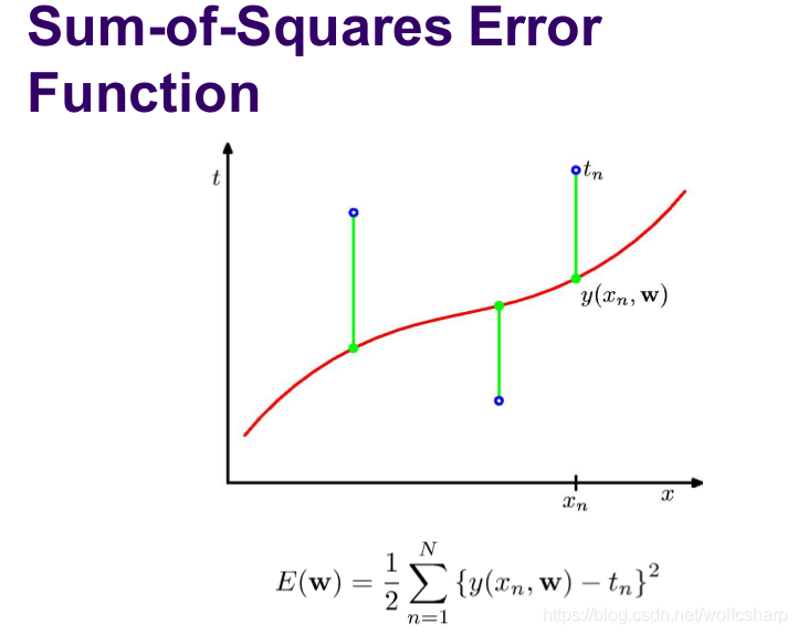
问题描述:给定一些数据点,用一个多项式尽可能好的拟合出这些点排布的轨迹,并给出解析解。判断拟合的好坏常用的误差衡量方法是均方根误差,要求均方根误差先要求平方和误差:
然后计算均方根误差:
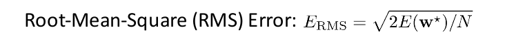
多项式拟合问题本质是一个优化问题,目标函数是使RMS误差最小。
本文关注于最小二乘法优化。
最小二乘法
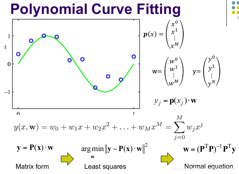
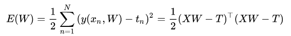
最小二乘法推导:RMS误差与E(W)成正比,E(W)最优等价于RMS最优
E(W):
对E(W)求导:
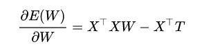
令导数=0:
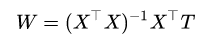
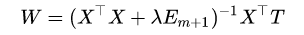
通过给定X和T,可以直接求得W,W就是多项式拟合中的系数矩阵。
针对overfitting,加入正则项
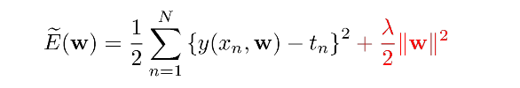
求导:
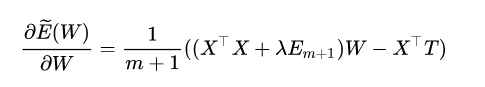
求出W:
python实现
注意: 在 colab中实现
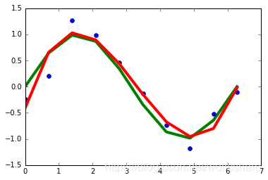
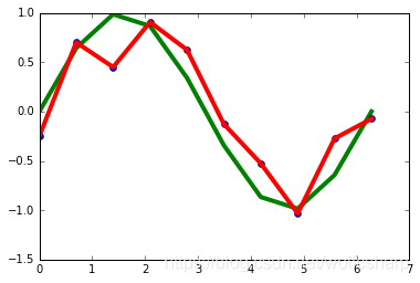
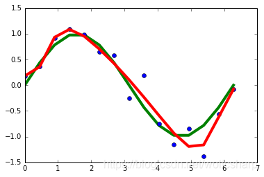
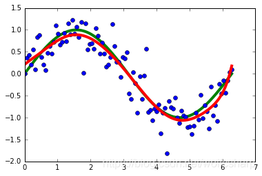
运行结果
绿色曲线 x-y
蓝色散点 x-y_noise
红色曲线 x-y_eatimate
-
sample number=10,3th
-
sample number=10,9th
-
sample number=15,9th
-
sample number=100,9th
-
sample number=10,9th 加入正则项

加入正则项会有效缓解overfitting问题。
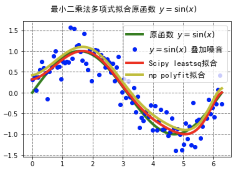
使用 Scipy中最小二乘函数leastsq 或者 numpy.polynomial.polynomial.polyfit 进行拟合
Scipy中optimize模块的leastsq函数:
一般只需要前三个参数就够了他们的作用分别是: - func:误差函数 - x0:表示函数的参数 - args()表示数据点
numpy.polynomial.polynomial.polyfit
参数: - x array_like,形状(M,) M个样本(数据)点的x坐标 - y array_like,形状(M,)或(M,K) - deg int或一维array_like
运行结果
sample number=100,9th
凡本网注明"来源:XXX "的文/图/视频等稿件,本网转载出于传递更多信息之目的,并不意味着赞同其观点或证实其内容的真实性。如涉及作品内容、版权和其它问题,请与本网联系,我们将在第一时间删除内容!
作者: Leo-Ma
来源: https://blog.csdn.net/wolfcsharp/article/details/89413244